PyMC in the browser, compiled to wasm
A while ago I wrote about stanwasm, a Stan subset that parses, compiles and samples inside the browser.
The part of it that compiles an autodiff tape to a WebAssembly module and has nuts-rs sample that module in the same memory, it occurred to me, could serve PyMC too.
So I pulled that part out into its own library, tapewasm, and connected PyMC to it as a second front end.
Here is PyMC actually sampling on the web.
The sampling runs in the browser, through wasm.
Larger models run too.
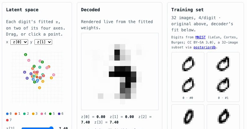
The next demo represents 32 MNIST digits with a small neural-network decoder from a four-dimensional latent variable to the pixels (4,344 parameters), and trains it in the browser by variational inference (mean-field ADVI).
The model is about ten lines of PyMC, built ahead of time into a wasm module with pymcwasm-build, so training runs in the page without loading Python.
- Open a JupyterLite notebook that installs PyMC and samples it, in your browser
- Open the MNIST decoder demo
 habakan/pymcwasmSample a PyMC model in the browser: the log density compiled to WebAssembly, drawn by nuts-rsgithub.comhabakan/tapewasmCompile a log density to a WebAssembly module and draw from it in the browsergithub.com
For now both are side projects of mine, not affiliated with PyMC.
PyMC's toolchain
In PyMC's toolchain, the automatic differentiation and much of the rest is done by PyTensor, a library maintained under pymc-devs.
PyTensor holds the model's computation as a graph and makes it fast by translating it into C, Numba or JAX and compiling that; it can also run on a GPU.
The part of PyTensor that decides what code a graph becomes is called a linker.
PyMC itself already runs on wasm
PyMC can in fact already run in the browser.
There are efforts like PyMC Labs' nuts-rs-wasm, which samples PyMC in the browser by shipping a dedicated Xeus / Emscripten environment that includes Numba.
This post is about the standard Pyodide instead, the one JupyterLite and marimo use to run Python in a page.
PyMC installs on Pyodide as it is.
What it loses on the wasm side is its compiler.
PyMC hands its log density to PyTensor, and PyTensor normally turns the graph into C and compiles it.
Pyodide has no C compiler. It is the same problem I described in "What to watch out for when putting Stan on wasm" last time: you cannot bring a compiler into the browser.
So PyTensor falls back to its Python linker and evaluates the graph one node at a time, in Python.
It works, but it does not get close to native performance.
On a logistic regression with 3,020 observations, PyMC's NUTS in a JupyterLite tab gets about one effective draw per second.
Using tapewasm for PyMC in the browser
So this time I tried to use tapewasm, an autodiff built with a wasm environment in mind, to make PyMC run faster on wasm.
There are two ways to use it.
The first way changes nothing about the model.import pymcwasm.linker registers a PyTensor linker called "WASM", and any PyTensor function can be compiled with it:
import pymcwasm.linker
await pymcwasm.linker.load(tapewasm_url)   # once per page, under Pyodide

with model:
    idata = pm.sample(compile_kwargs={"mode": "WASM"})
PyMC's own NUTS still runs, in Python.
What changes is that every log density and gradient it asks for is a call into a WebAssembly module instead of a walk over the graph.
The second way goes further.
Once the density is fast, most of what is left is PyMC's sampler itself, stepping in Python.pymcwasm.sample compiles the same density once and hands the whole sampler to the module as well, so no Python runs per step:
fit = await pymcwasm.sample(model, draws=500, warmup=500, chains=2)
idata = fit.to_inference_data()
On the notebook's eight schools model, two chains of a thousand iterations each:
| time in the page | |
|---|---|
| PyMC's NUTS, PyTensor's Python linker | 5.8 s |
PyMC's NUTS, mode="WASM" |
1.2 s |
pymcwasm.sample |
0.02 s, after 0.21 s compiling |
How it works
A PyMC model is a PyTensor graph.
pymcwasm writes that graph out as a "tape", a list of scalar operations like additions and multiplications, with the data folded in as constants.
tapewasm turns the tape into a wasm module that returns the log density and its gradient together in one call.
The sampler, nuts-rs, calls that module in the same memory, so one gradient is one function call with no data copied.
For a small model the module is 5 to 35 KB, and built ahead of time it can go on a page that never loads Python (the MNIST demo is built that way).
There is one constraint. A tape has no branches like an if, so a comparison such as sigma > 0 is fixed to whatever it was when the tape was written.
So on every call the module also checks whether those comparisons still come out the same, and if one does not, the tape is written again.
I check correctness against posteriordb: of its 83 posteriors with a PyMC implementation, 79 agree with PyMC on the log density and gradient (the other four use operations I have not covered yet). That check runs in CI.
Measuring performance
To see the shape across sizes, I ran nine posteriordb posteriors, from 2 to 3,075 parameters, under five samplers: three in a Pyodide worker in Chromium, and PyMC's NUTS and nutpie on CPython for comparison.
Each gets two chains of 500 warmup and 500 draws and is scored by the smallest bulk ESS per second of sampling, on an Apple M3.
| model | params | Pyodide, Python linker | Pyodide, mode="WASM" |
Pyodide, pymcwasm.sample |
CPython, PyMC NUTS | CPython, nutpie |
|---|---|---|---|---|---|---|
| eight schools | 10 | 76 | 719 | 3,944 | 2,213 | 21,333 |
| arK | 7 | 35 | 259 | 1,178 | 685 | 4,545 |
| radon, varying intercept | 89 | 11 | 114 | 345 | 326 | 2,015 |
| wells, logistic | 2 | 1.0 | 98 | 148 | 285 | 402 |
| radon, 12,573 observations | 391 | 0.3 | 4.7 | 5.5 | 16 | 78 |
In the page, mode="WASM" is 10 to 100 times the Python linker.pymcwasm.sample keeps up with PyMC's NUTS on CPython up to about a hundred parameters, which I did not expect.
It does not keep up with nutpie, which is 3 to 10 times faster there, and the gap grows with the data: 3 to 15 times on the large-N models.
The module is a tape of scalars, where nutpie runs numba's vectorised loops, and that difference is what a large dataset exposes.
The full tables and the harness are in bench/.
What it cannot do yet
Scan is not lowered, so no state-space models.
A branch on a parameter that is a real branch and not a bounds check is guarded rather than compiled, so it works but retraces.Maximum, BetaInc and discrete parameters are missing, and there is no posterior predictive inside the module.
And large data costs module size and speed, as above.
Closing
To make PyMC fast in the browser, I wrote PyTensor's graph onto an autodiff tape and called it as a wasm module.
On standard Pyodide, adding mode="WASM" makes PyMC's NUTS faster, and handing the sampler to the module as well puts it level with native PyMC up to about a hundred parameters.
Next I want to work on speed with large data. If the tape could keep vector operations as vectors instead of a list of scalars, the gap to nutpie should narrow.
If you teach with JupyterLite, or have a model you would like to put in a page without a server, I'd like to hear whether this is useful, and where it breaks.